Electromagnetic induction is by no means a straight forward topic to get your head around whether you study Physics or not. It comes with a lot of terminology, definitions and understanding of magnetic fields and their interaction with motion.
Last period on Friday (after the students’ first week back after the Summer holiday), the students needed to get some blood flowing after recapping and learning the definitions for magnetic flux density, magnetic flux and magnetic flux linkage, which I have outlined here if you are interested:
Magnetic Flux Density – what is it?
Magnetic flux density is defined as the the force exerted per Ampere per length. It enables us to exert a force on a wire carrying when it is inside a magnetic field. This are of physics is pivotal for understanding how to get motors running, wheels turning and in general things moving.
The equation for magnetic flux density is:
where; B is the magnetic flux density, measured in Tesla’s, T F is the force acting on the conductor, measure in Newtons, N I is the current in the wire within the magnetic field, measured in Amps, A
L is the length of the conductor within the magnetic field, measure in metres, m
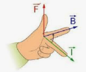
If you have studied this you will also have come across Fleming’s Left Hand rule: used to determine the direction acting on the current carrying conductor.
It is important to remember Newton’s 3rd law of motion: Every action has an equal and opposite reaction. This tells us that although a force is acting on the wire, an equal and opposite force will act on the magnet.
Magnetic Flux – what is it?
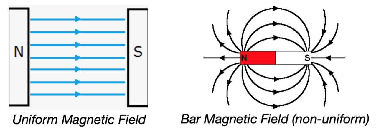
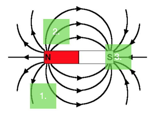
Magnetic Flux is an important concept because it helps us to understand how the field changes from one location to another. In a uniform magnetic field the strength of the field (known as magnetic flux density) is constant, but around a bar magnet it varies: The distance between the field lines helps to demonstrate the strength of a field. For the uniform field, the fields lines are equally spaced and so the strength is equal in all areas within that region. For the bar magnet, the lines get closer or further apart depending on the position. The strongest region will be at the poles. If we focus on the bar magnet and take a a certain sized cross sectional area and moved it around the field we can begin to see this clearly:
Position 1 shows 2 lines within the area (just about).
The position 2 displays 3 lines passing through the region, so more than position 1 and therefore the field is strong here.
On the right hand side, position 3 has many lines going through it, so the field is much stronger here.
This idea of the number of field lines is one way to think of ‘flux’. It is how strong the field is within a given area. If we made the area bigger there would clearly be more field lines that would pass through it, so the magnetic flux would increase. If we kept the area the same but increased the strength of the field then there would be more field lines and so again the magnetic flux would increase.
Magnetic flux is therefore defined as the the product of the magnetic flux density and the area perpendicular to the field. As an equation we can write:
where; ϕ is the magnetic flux, measured in Webers, Wb
B is the magnetic flux density, measured in Tesla’s, T
A is the cross sectional area in which the magnetic field lines pass through, measure in metres square, m²
In reality, the cross sectional area may not be perpendicular to the field and therefore the full equation to use differs:
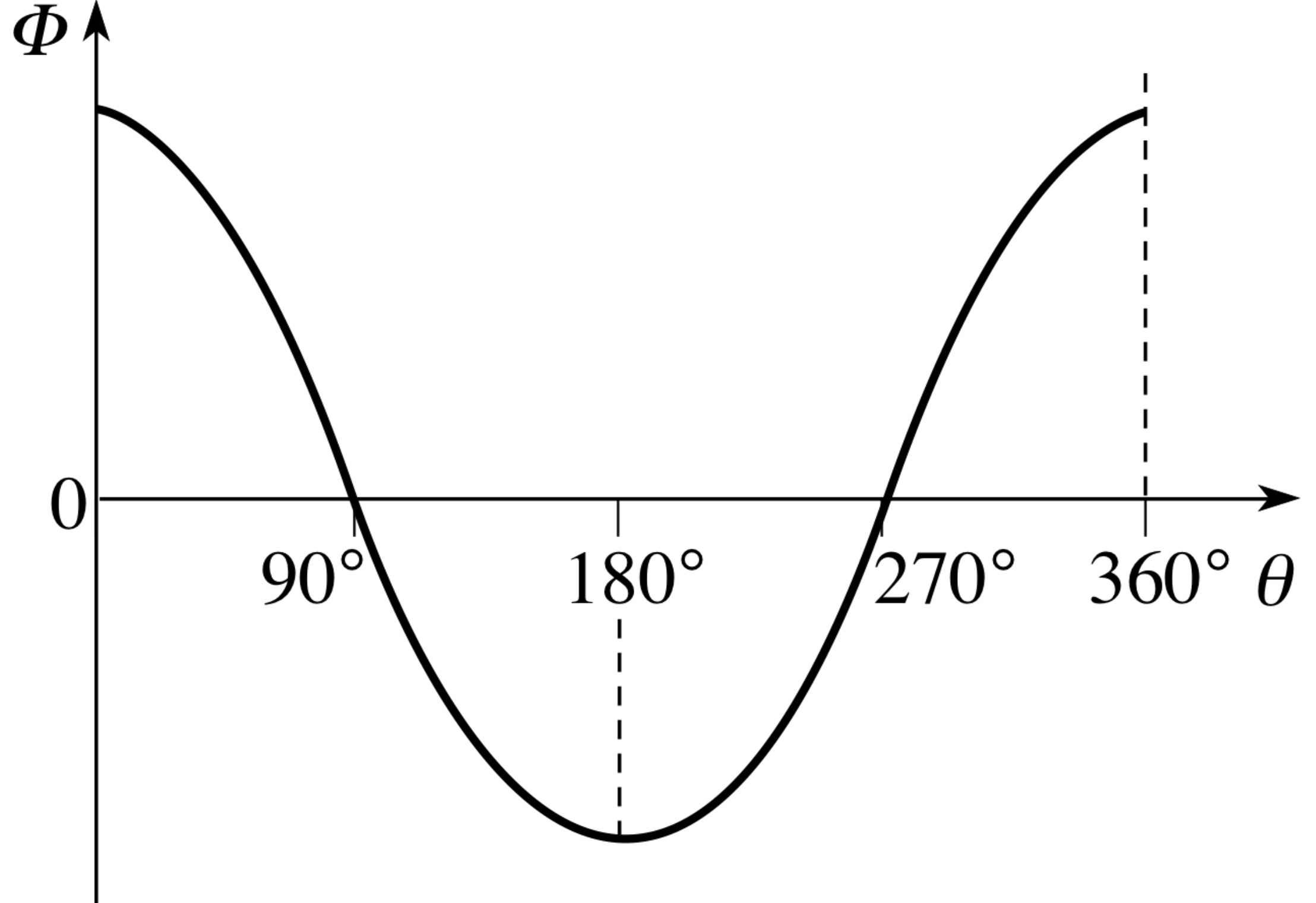
If the cross sectional area is perpendicular to the field we can say the angle is correct and so θ = 0°. In this position most field lines will pass through the area and so the magnetic flux will be a maximum.
If the cross sectional area is parallel to the field, we can say the angle is 90° to the perpendicular. Int this position no field lines would pass through the field and so the magnetic flux will be a minimum (or zero).
If we continue to turn the cross sectional area by a further 90°, the area would return to being perpendicular to the field (but now the field lines would go through it in the opposite direction). The magnetic flux would therefore be a maximum again, but negative to account for the different direction.
This creates a cosine graph. This results in the equation for magnetic flux changing to:
Magnetic Flux Linkage – what is it?
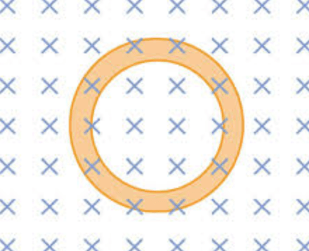
Magnetic flux linkage is where this terminology links to electromagnetic induction. If we introduce a wire to a magnetic flux and shape it into a circle encompassing an area, then we have linked with the magnetic flux – hence the term magnetic flux linkage.
Take this gold ring as an example: It is metal and in a loop, there is a magnetic field within the ring (shown by the crosses – which represent that the field is going into the screen). The area within the ring represents the cross sectional area.
We can link more rings (or more wire) to the magnetic field by turn the wire into more circles (or having more rings).
For each turn in the wire, we have linked another loop to the magnetic flux. The equation for magnetic flux linkage is therefore equal to BAN, if we take the shorter version of the equation for magnetic flux. The N stands for the number of turns in the wire. If we doubles the number of turns we would double the magnetic flux linkage because we would have twice the number of electrons linking with the magnetic flux.
The equation is written as:
There is no official symbol for magnetic flux linkage, and so we take the product of magnetic flux and the number of turns to represent it – therefore we don’t just cancel off the N’s from both sides.
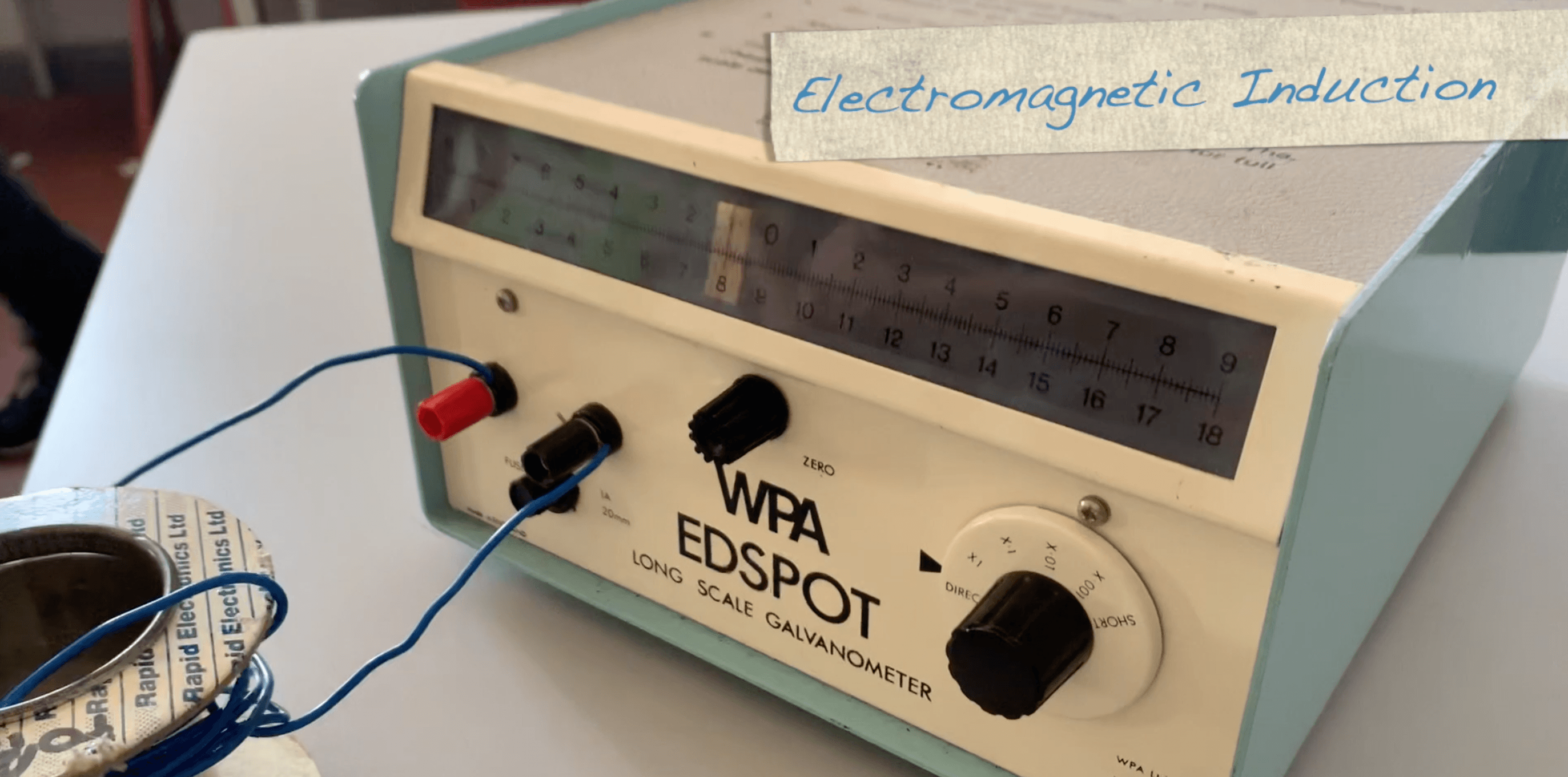
The students took a long wire (approximately 15 m in length) made a loop where both ends were connected to a galvanometer, this is an instrument used for detecting very small electrical currents. Putting it simply, they held in their hands a long wire in one big loop connected to an ammeter and nothing else.
To the Hokey Cokey song, the moved in and out, shaking that wire all about! See what happened to the ammeter.
What they learned was that they were linked with the magnetic field of Earth!
By completing a loop and connecting it to the galvanometer, they were able to induce an e.m.f, thereby forcing a current into the wire. How cool is that?!
Earths magnetic field is tiny and about 50 μT, yet we can see its affects in a classroom by doing a little dance!
If their faces weren’t blurred you would be able to see how much fun they were having! I almost got them to do this on the playground, but felt that the sixth formers may never want to show up to my lesson again.
Explaining these observations
By linking the wire to the galvanometer and moving in and out of Earths magnetic field they were inducing an e.m.f. When they were stationary, the galvanometer was stationary showing no signs of an induced e.m.f. This should make sense to us as without their input of energy, they would not have been able to induce a form of electrical energy (conservation fo energy).
So the magnetic flux linkage induced an e.m.f. WHEN they moved through the field. Michael Faraday observed this in 1831 and wrote a law to explain things:
The e.m.f induced is proportional to the rate of change in magnetic flux linkage. As an equation he wrote this as:
That… was where we ended the lesson. I’m looking forward to reviewing it and getting them to learn Lenz’s law next!
The only thing that interferes with my learning is my education.


 The students took a long wire (approximately 15 m in length) made a loop where both ends were connected to a galvanometer, this is an instrument used for detecting very small electrical currents. Putting it simply, they held in their hands a long wire in one big loop connected to an ammeter and nothing else.
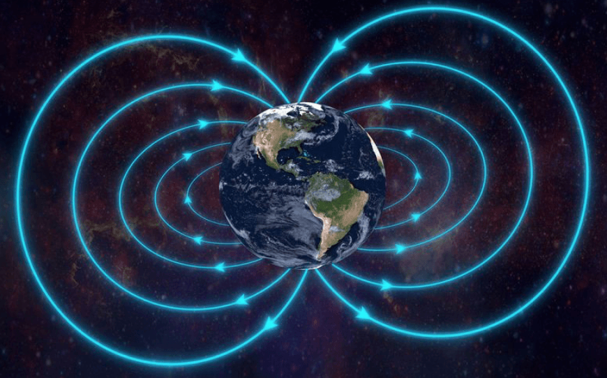 By completing a loop and connecting it to the galvanometer, they were able to induce an e.m.f, thereby forcing a current into the wire. How cool is that?!