4. Electrical Potential - Motion of Charged Particles : Educating Physics

Objectives:

To understand equipotential lines are and how they can be used
To understand the motion that charged particles undergo when in a uniform electric field
To practice the use of equations and calculations on topics studied so far
To apply the equations of motion to particles in a uniform electric field

We know that the electric field between two parallel plates is uniform and the strength of this field is dependent on both the potential difference between the plate and the separation of the plates.

Equipotential lines

Equipotential lines are drawn as dashed lines that, especially for a uniform electric field, are drawn perpendicular to the electric field lines. These equipotential lines represent where the electric potential in that field is the same. For example, in the following image equipotential lines are drawn to divide the total potential difference between the plates up into smaller sections.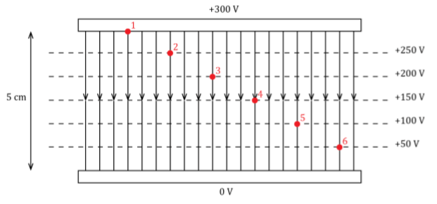

In this particular example, the equipotential lines dived the p.d up into $50 \ V$ sections, but the physicist using the diagram can in fact split them up into whatever magnitude they want (i.e they could separate every $100 \ V$ instead).

Contour lines

Equipotential lines are similar in a way to contour lines on a map.

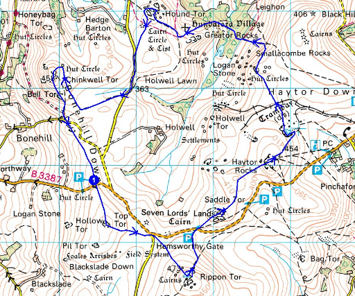
The contour lines represent the height above sea level. If you were to walk along one of these contour lines you would never do any work against gravity and therefore would always have the same gravitational potential energy. The following image perhaps shows this more clearly:

Image taken from: https://gisgeography.com/contour-lines-topographic-map/

Instead of the amount of energy against gravitational field, equipotential lines refer to the an amount of energy against an electrical field. So going back to the following example:

Let’s pretend we drop a proton in different positions within the two plates.

This proton will accelerate towards the $0 \ V$ plate as it is the negative terminal. Using $E = \frac{F}{q}$ and $E = \frac{V}{d}$ , we can equate them to get:

$\frac{F}{q} = \frac{V}{d}$

Since $F = ma$ , this too can be substituted in to give:

$\frac{ma}{q} = \frac{V}{d}$

By rearranging this for $a$ we can determine the magnitude of the acceleration exerted on this proton:

$a = \frac{qV}{md}$

where:
$a$ is the acceleration
$q$ is the charge of the particle within the field
$V$ is the potential difference between the plates
$m$ is themass of the particle within the field
$d$ is the separation of the plates.

Determining the final velocity of a particle within an electric field

The particle placed within the field (in this case a proton), will accelerate in the same direction as the force which can be determined by looking at the direction of the electric field lines (and whether the charge is positively or negatively charged).

The following questions will assume that the proton is placed, initially stationary, at positions 1-6 individually:

If placed initially stationary the final velocity can be calculated by using the equations of motion, this is because between parallel plates the the electric field is uniform and therefore there is constant acceleration.

Determining the acceleration:

$a = \frac{qV}{md}$

$a = ?$ is the acceleration
$q = 1.6 \times 10^{-19} \ C$ is the charge of the particle within the field
$V = 300 \ V$
$m = 1.673 \times 10^{-27} \ kg$
$d = 5 \ cm = 0.05 \ m$

Substituing these into $a = \frac{qV}{md}$ gives:

$a = \frac{1.6 \times 10^{-19} \times 300}{1.673 \times 10^{-27} \times 0.05} = 5.738 \times 10^{11} \ ms^{-2}$

Position 1:
We know the acceleration (or at least we can calculate it), the distance it travels, and the initial velocity is $0 \ ms^{-1}$ . Using the equation $v^{2} = u^{2} + 2as$ , we can calculate the final velocity, $v$ . One thing to be careful about is that the distance $s$ is not always the distance between the plates but the distance traveled by the particle, for position 1 it is the same however.

$s = 5 \ cm = 0.05 \ m$
$u = 0 \ ms^{-1}$
$v = ?$
$a = 5.738 \times 10^{11} \ ms^{-1}$
$t = \text{unknown}$

$v^{2} = u^{2} + 2as$

$v^{2} = 0 + 2 \times 5.738 \times 10^{11} \times 0.05$

$v^{2} = 5.738 \times 10^{10}$
$v = 2.395 \times 10^{5} \ ms^{-1}$
$v = 2.4 \times 10^{5} \ ms^{-1}$ (2 s.f.)

Energy gained by the charged particle:

Now that the final speed is known the energy gained by the proton can also be deduced. Since it has accelerated, it has gained kinetic energy, so the energy gained is equal to $\frac{1}{2} mv^2}$

$E = \frac{1}{2} \times 1.673 \times 10^{-27} \times (2.395 \times 10{5})^{2}$
$E = 4.798 \times 10^{-17} \ J$
$E = 4.8 \times 10^{-17} \ J$ (2 s.f.)

There is an alternate method for working out the energy gained by the charged particle, this is by using the definition of potential difference, $V = \frac{W}{q}$ :

Since the potential difference between the charged particle at the $0 \ V$ plate is $300 \ V$ , the work done on the charged particle through a distance of $d = 0.05 \ m$ is:

$W = Vq = 300 \times 1.6 \times 10^{-19} = 4.8 \times 10^{-17} \ J$

As you can see from the two results, they are the same, and they correspond to the potential difference between the plates, as it is defined as the work done n a charge.

As you have seen from your AS modules, an amount of energy this small is usually written in electronvolts, so:

$\frac{4.8 \times 10^{-17}}{1.6 \times 10^{-19}} = 300 \ eV$

Notice how the amount of energy, $300 \ eV$ is the potential difference between the charged particle and $0 \ V$ plate – this should be obvious as we have just done that exact calculation above.

The other 5 positions:

We are now going to calculate the same values (final speed, energy in joules and energy in eV) for a proton dropped in the other five positions indicated in the same diagram (shown again below), without showing the calculations. If in doubt, check with the above ones, the only variable that changes is the distance (not between the plates, but the one traveled by the particle).

Try doing your own calculations first and then check the table below to see if you are correct. A second example showing position 2 is done below the table.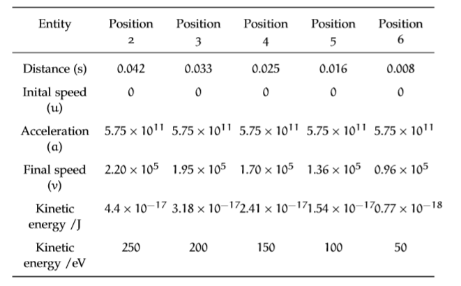

As you can see from Table, the final answer in electron volts are the same values as the equipotential lines drawn.

Example for position 2

Acceleration:
This is the same as for position 1 since the field is uniform, $a = 5.738 \times 10^{11} \ ms^{-2}$

Final speed:
$s = \frac{5}{6} \times 5 \ cm = 0.05 \ m$ (notice this has changed as the particle is not travelling as far)
$u = 0 \ ms^{-1}$
$v = ?$
$a = 5.738 \times 10^{11} \ ms^{-1}$
$t = \text{unknown}$

$v^{2} = u^{2} + 2as$
$v^{2} = 0 + 2 \times 5.738 \times 10^{11} \times (\frac{5}{6}) 0.05$
$v = 2.2 \times 10^{5} \ ms^{-1}$ (2 s.f.)

Kinetic energy:
$E = \frac{1}{2} m v^{2}$
$E = \frac{1}{2} \ times 1.673 \times 10^{-217} \times (2.2 \times 10^{5})^{2}$
$E = 4.0 \times 10^{-17} \ J$
$E = \frac{4.0 \times 10^{-17}}{1.6 \times 10^{-19}} = 250 \ eV$