Objectives:
- To understand Kirchhoff’s second law; the conservation of energy
- To understand how Kirchhoff’s first and second laws apply to electrical circuits
Recap on Kirchhoff’s first law
Kirchhoff’s first law, also known as Kirchhoff’s current law (KCL) states that;
The sum of the currents entering a junction must be equal to the sum of the current leaving that same junction – this is a conservation of charge.
A complete recap of Kirchhoff’s first law can be found by going to the page: 3. Kirchhoff’s 1st Law
Take the following diagram;
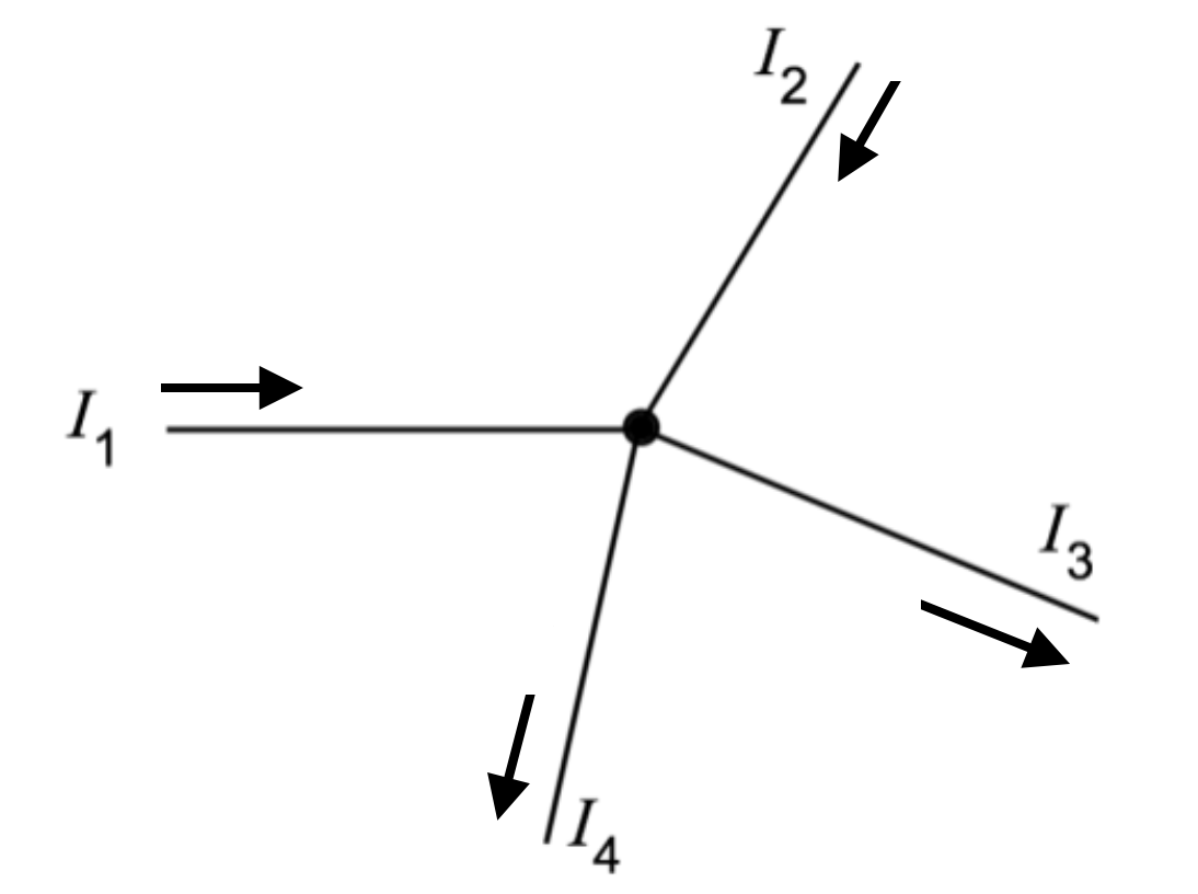
The following equations can be written regarding the current flow;

Or from the right of the trio of resistors we could write;

Kirchhoff’s second law
Kirchhoff’s second law is also known as Kirchhoff’s voltage law (KVL) and focuses on the e.m.f. supplied to a circuit as well as the p.d.
Series circuits

If we take this simple circuit here;
When the switch is closed a current is free to flow due to the e.m.f. supplied by the cell. The energy per unit charge (voltage) is then given and used by the bulb. The energy supplied by the cell will be equal to the energy used by the bulb. Therefore;

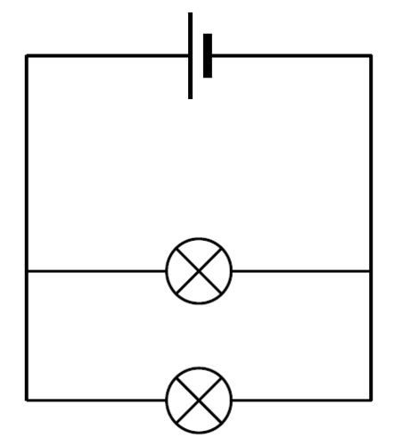
If we supply two bulbs instead of one;
 With a complete circuit, the energy per unit charge (voltage) supplied by the cell has to be distributed to the two bulbs (the distribution will depend on the resistance of each bulb – but this will be covered in more depth at a later stage). Some of the e.m.f. will supply the first bulb with a p.d. and some will provide the second bulb with a p.d. Therefore;

The electrons carry the energy and must distribute it across the two bulb. If the first bulb has more resistance, then it will use a greater amount of the p.d. in which case it may shine more brightly, and vice versa.
Parallel circuits
If we take this simple parallel circuit;
When the circuit is complete, the cell provides every unit of charge with an amount of energy (voltage) (take a unit of charge to be a single electron). Every ‘electron’ (or unit of charge) that passes through the cell gains a amount of energy, E, when the the electrons get to the junction some will travel along to the upper bulb (1) and the other will travel to the lower bulb (2). BUT, the amount of energy each electron has does not split only the number of electrons themselves.
Therefore, the current divides but the voltage (or energy each electron has) stays the same.
We can therefore write;
Take the following circuit;
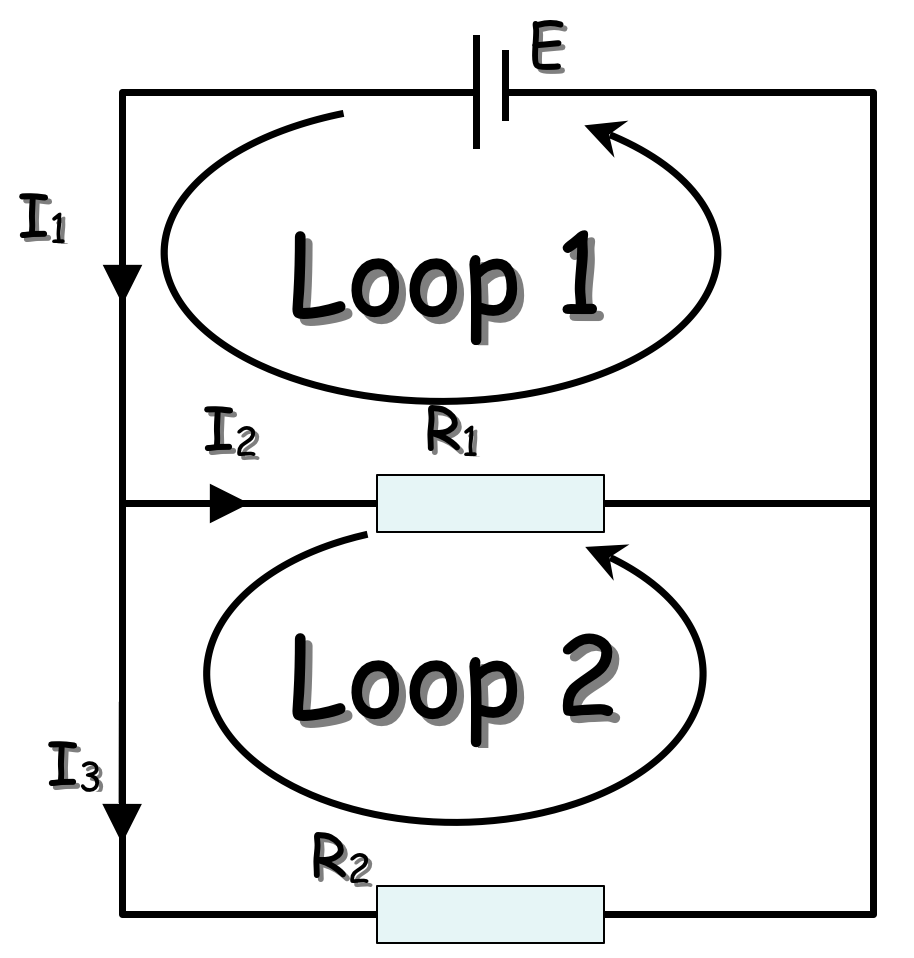
The e.m.f supplied to loop 1 is equal to the p.d. of loop 1. Similarly the e.m.f. supplied to loop 2 (which comes from the cell) is equal to the p.d. of loop 2.
We can therefore write that the sum of the e.m.f. of a loop is equal to the sum of the p.d.’s in that same loop – this is the conservation of energy.
It can also be written as;
Kirchhoff’s voltage law states that the sum of all voltages around any closed loop in a circuit must equal zero.
Using the last circuit we can now write several equations that satisfy Kirchhoff’s first and second law.
Using KCL:

Using KVL: 
We can now use the definition of resistance to help us expand KVL equation further;

The voltage through resistor 1 is dependent on the current 


Similarly for $R_{2} $ we can write;

Subbing equations (2) and (3) into equation (1) gives;

This tells us that both 

Further equations can be constructed by using KCL or by exchanging the e.m.f for 
Further reading:
- Isaac Physics – Kirchhoff’s Law – This is a reading resource
- Kirchhoff is an important figure in physical and chemical science; you could do background research on his life and achievements.
- Parallel Circuits from http://www.physicsclassroom.com/
You must be logged in to post a comment.